Simulating protein-peptide complex and predicting native state
Introduction
Here we will learn how to setup a protein-peptide system and run simulation and analyze the trajectory to predict the native complex structure. For that we will start the simulation from unbound conformation of both receptor (protein) and ligand (peptide) and allow data and force field to guide to the native bound conformation of the complex. Here we will work with a known protein complex of ET domain of BRD3 protein with MLV peptide (RCSB PDB code 7jq8). Unbound form of BRD3 ET protein is also available as PDB code 7jmy. Here this tutorial is done with meld/0.6.0 version.
Setup of the starting system
The protein sequence is
HHHHHHSHMGKQASASYDSEEEEEGLPMSYDEKRQLSL DINRLPGEKLGRVVHIIQSREPSLRDSNPDEIEIDFET LKPTTLRELERYVKSCLQKK
where first 28 residues are purification tag. So we will exclude that in the simulation and we have
SYDEKRQLSLDINRLPGEKLGRVVHIIQSREPSLRDSN PDEIEIDFETLKPTTLRELERYVKSCLQKK
and the peptide sequence is
SRLTWRVQRSQNPLKIRLTREAP
Since we want to start from a free peptide conformation, we generate a minimized PDB file for the peptide in an extended conformation. We can use setup_from_random. sh script in this directory for this purpose. This script uses ‘setup_system’ function to generate tleap input. Then tleap generates topology and initial coordinate which we minimize using amber to generate a minimized pdb for the peptide. The ‘setup_system’ script follows as:
def setup_system():
    # load the sequence
    sequence = meld.get_sequence_from_AA1(filename='sequence.dat')  # above mentioned peptide sequence is in sequence.dat file
    n_res = len(sequence.split())
    # build the system
    p = meld.AmberSubSystemFromSequence(sequence)
    b = meld.AmberSystemBuilder(forcefield="ff14sbside")   # we use ff14SB side and ff99SB backbone forcefield
    s = b.build_system([p]).finalize()            # build the pdb file
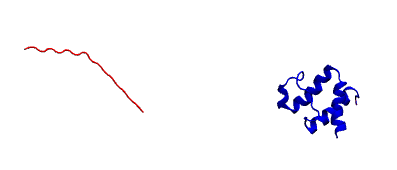
We will combine this minimized peptide pdb and unbound protein pdb (minimized as well) together. One thing we have to make sure is that peptide is atleast 30 angstrom far away from the receptor. There are several ways to shift coordinate of either receptor or peptide. Using change_coor.py script is one of the ways. Finally we have minimized_complex.pdb. A ascreenshot of the starting system from vmd is given below.
Prepare the input restraint file for this system:
As we already learned, MELD is based on Bayesian frameworks, it uses data coming from all sort of sources and an atomistic force field. Data plays a major role here, it helps to limit the conformational landscape and help to find minima faster. The principle of MELD is explained in detailed somewhere else.
For this particular example we will use distance restraints between protein-peptide residue pairs. Since the structure is known, we use the native complex structure to determine protein-peptide CA pairs which are within 8 angstrom from each other and use those in the simulation to guide the binding. This protein-peptide restrain file is added here as protein_pep_all.dat which is calculated using popular python library MDTraj and the script is also given here as pdb_contacts.py. Few restraints from this file are shown here:
5 CA 82 CA 0.5846176743507385
6 CA 81 CA 0.5934389233589172
6 CA 82 CA 0.5739095211029053
9 CA 81 CA 0.6932587623596191
…
…
Here, residue 1 to 68 is corresponding to the protein and 69 to 91 for peptide. The first column is residue number of protein and second column is atom in protein residue, 3rd and 4th column are respectively residue number and atoms for peptide and the 5th column is the distance between those two atom in nanometer. To be specific, the 1st row means CA of 5th residue should be 7.5 angstrom away from CA of 82nd residue (which is 82-68=14th residue in peptide) in the bound conformation. These restraints are mere for tutorial purposes, for real system we need to get data from experiment or statistical analysis as complex structure will be unknown. Also one gap between each restraints are importants for this particular simulation setup as we are defining all these restraints as a collection, and inside collection we have groups seperated by blank line and in each group we have restriants. Here each group only has one restriant.
We are using unbound protein conformation in our simualtion, the protein will probably go through conformational change upon complex formation- but we can expect it keep its fold intact. For this, we calculate interprotein residue pairs within 8 angstrom and put distance restraints on them in a similar way to peptide. We can use similar script for this purpose as well and it generates protein_contacts.dat file.
Setup of the MELD simulation
At this point if we have the following files, we are ready to setup a simulation–
minimized_complex.pdb in the /TEMPLATES directory #starting structure
protein_contacts.dat #restraints to keep recpetor folded
protein_pep_all.dat #restraints to guide binding
setup_MELD.py #python script to setup the simulation.
By this point we are familiar with all three files except setup_MELD.py. This is a python script which is creates the platform of the simulation we are going to carry out. With this we read the restraint files, generate the initial states for each replica at different temperature and hamiltonial (force constant/ restraint strength) and launch OpenMM jobs associated with replica exchange protocol. Here is how we write the file:
We first import some necessary python modules:
import numpy as np
import meld
import glob as glob
Then we define some important parameters:
N_REPLICAS = 30  # Number of replicas
N_STEPS = 2000   # Total step of simulaion.
BLOCK_SIZE = 100 # Save the trajectory in 'chunk' of 100 frames.
Then some functions to generate intial state and read the restraint files:
def gen_state_templates(index, templates): # to generate the initial state
    n_templates = len(templates)
    print((index,n_templates,index%n_templates))
    a = system.ProteinMoleculeFromPdbFile(templates[index%n_templates])
    #Note that it does not matter which forcefield we use here to build
    #as that information is not passed on, it is used for all the same as
    #in the setup part of the script
    b = system.SystemBuilder(forcefield="ff14sbside")         #using ff14SB backbone and ff99SB sidechain force field
    c = b.build_system_from_molecules([a])
    pos = c._coordinates
    c._box_vectors=np.array([0.,0.,0.])
    vel = np.zeros_like(pos)
    alpha = index / (N_REPLICAS - 1.0)
    energy = 0
return system.SystemState(pos, vel, alpha, energy,c._box_vectors)

def get_dist_restraints(filename, s, scaler):             # to read the binding restraints
    dists = []
    rest_group = []
    lines = open(filename).read().splitlines()
    lines = [line.strip() for line in lines]
    for line in lines:
        if not line:
            dists.append(s.restraints.create_restraint_group(rest_group, 1))                    # enforcing 1 restraints from each group
            rest_group = []
        else:
            cols = line.split()
            i = int(cols[0])
            name_i = cols[1]
            j = int(cols[2])
            name_j = cols[3]
            dist = float(cols[4])                          # MELD uses nm unit for distance

            rest = s.restraints.create_restraint('distance', scaler,LinearRamp(0,100,0,1),       #Flatbottom harmonic restraints with no poteintial from 0 nm (r2) to 'dist' (r3) in the given in the file and then r3 to r4 increaing harmonically and after that increasing lineraly with k=350 kJ/(mol.nm*2)
                                              r1=0.0, r2=0.0, r3=dist, r4=dist+0.2, k=350,
                                              atom_1_res_index=i, atom_2_res_index=j,
                                              atom_1_name=name_i, atom_2_name=name_j)
            rest_group.append(rest)
return dists


def get_dist_restraints_protein(filename, s, scaler):                   #To read the restraint to keep protein conformation fixed
    dists = []
    rest_group = []
    lines = open(filename).read().splitlines()
    lines = [line.strip() for line in lines]
    for line in lines:
        if not line:
            dists.append(s.restraints.create_restraint_group(rest_group, 1))
            rest_group = []
        else:
            cols = line.split()
            i = int(cols[0])
            name_i = cols[1]
            j = int(cols[2])
            name_j = cols[3]
            dist = float(cols[4])

            rest = s.restraints.create_restraint('distance', scaler,LinearRamp(0,100,0,1),
                                              r1=dist-0.2, r2=dist-0.1, r3=dist+0.1, r4=dist+0.2, k=350,      # here we have 0 energy penalty in betwen dist-0.1 and  dist+0.1 region making it stronger contact.
                                              atom_1_res_index=i, atom_2_res_index=j,
                                              atom_1_name=name_i, atom_2_name=name_j)
            rest_group.append(rest)
return dists
Now that we have defined all the required function, it is time to call them. Here is how we do it.
def setup_system():
    templates = glob.glob('TEMPLATES/*.pdb')       # read the template file, can be multiple
    p = system.ProteinMoleculeFromPdbFile(templates[0])         #build the system
    b = system.SystemBuilder(forcefield="ff14sbside")           # use force field
    s = b.build_system_from_molecules([p])
    s.temperature_scaler = system.GeometricTemperatureScaler(0, 0.4, 300., 500.)   #setup temperature range 300K to 500K for replicas. 0 is for the first replcia and 0.4 is for 30*0.4= 12th replica i.e. we assign temperature from 300 to 500K on first 12 replicas and then contast 500K for rest. This temperature range is distributed geometrically over 12 replcias.
    n_res = s.residue_numbers[-1]       #length of the system


    prot_scaler = s.restraints.create_scaler('constant')              # defining a constant distance scaler i.e. it will keep restraint strength equal through the replica ladder
    prot_pep_scaler = s.restraints.create_scaler('nonlinear', alpha_min=0.4, alpha_max=1.0, factor=4.0)   # Defining a nonlinear distance scaler. 1st to 12th replica will have maximum restraint strength and then from 12 to 30th it will decreas making 0 at the 30th


    prot_pep_rest = get_dist_restraints('protein_pep_all.dat',s,scaler=prot_pep_scaler)  # Enforcing binding restraints with non-linear scaler assignig high temperature replicas weaker restraints so that they can explore the energy landscape.
    s.restraints.add_selectively_active_collection(prot_pep_rest, int(len(prot_pep_rest)*1.00))   # Trusting all the groups in the restraint file

    prot_rest = get_dist_restraints_protein('protein_contacts.dat',s,scaler=prot_scaler)        #Enforcing intra protein restraints with constant scaler so that it does not unfold.
    s.restraints.add_selectively_active_collection(prot_rest, int(len(prot_rest)*0.90))        # Trusting 90% the groups in the restraint file providing flexibility to the receptor.

    options = system.RunOptions()
    options.implicit_solvent_model = 'gbNeck2'         #implicit solvent gbNeck2 model
    options.use_big_timestep = False
    options.use_bigger_timestep = True
    options.cutoff = 1.8

    options.use_amap = False
    options.amap_alpha_bias = 1.0
    options.amap_beta_bias = 1.0
    options.timesteps = 11111                          #We save 1 frame in each 11111 frames, i.e. every 50 ps
    options.minimize_steps = 20000
    options.min_mc = None
    options.run_mc = None
    ### here we define some important parameters which are with their optimized values
    # create a store
    store = vault.DataStore(s.n_atoms, N_REPLICAS, s.get_pdb_writer(), block_size=BLOCK_SIZE)
    store.initialize(mode='w')
    store.save_system(s)
    store.save_run_options(options)

    # create and store the remd_runner
    l = ladder.NearestNeighborLadder(n_trials=100)
    policy = adaptor.AdaptationPolicy(2.0, 50, 50)
    a = adaptor.EqualAcceptanceAdaptor(n_replicas=N_REPLICAS, adaptation_policy=policy)

    remd_runner = leader.LeaderReplicaExchangeRunner(N_REPLICAS, max_steps=N_STEPS, ladder=l, adaptor=a)  #launching replica exchange
    store.save_remd_runner(remd_runner)

    c = comm.MPICommunicator(s.n_atoms, N_REPLICAS)               # create and store the communicator
    store.save_communicator(c)

    states = [gen_state_templates(i,templates) for i in range(N_REPLICAS)]         # create and save the initial states
    store.save_states(states, 0)

    # save data_store
    store.save_data_store()

    return s.n_atoms

setup_system()
Now we know how setup_MELD.py file looks like. WIth all the abovementioned files in the working director, next step is to execute this file:
python setup_MELD.py
This will create a /Data directory in the working direcotry with following files and folder:
Backup/ Blocks/ communicator.dat data_store.dat remd_runner.dat run_options.dat system.dat
Backup directory has information needed for restarting the simulation if fails in between and /Blocks direcotry has those ‘chunk’ trajectories of 100 frmaes.
At this point we are ready to launch the simulation. This will be done using:
srun --mpi=pmix_v3 launch_remd --debug #it might chnage depending on the cluster we are using
Notice that we are launching a mpi job. Here we use 30 GPUs in mip manner with 1 GPU for each replica. We need to submit this in queueing system.
If the job fails before finishing, we can restart it by first executing following command:
prepare_restart –prepare-run
Then resubmitting the previous submission script.
Once the job start to run, it will generate trajectory.pdb in /Data directory with all the saved frame of the lowest temperature replica which we can visualize with any visualization tool and it will also generate remd.log file with the real time progress of the simulation.
Analysis
When the simulation is completed i.e. run for the intended steps, we can do several analyses. We have 30 replicas in our simulation and they exchnage at certain interval assing them different temperature and force constant. We can extract those 30 trajectories along the temperature range and as well as force constant range using the following command:
extract_trajectory extract_traj_dcd –replica 0 trajectory.00.dcd # to extract the 1st temperature replica i.e. lowest temperature replica
extract_trajectory extract_follow_dcd –replica 0 follow.00.dcd # To extract the 1st walker which walks through different temperature.
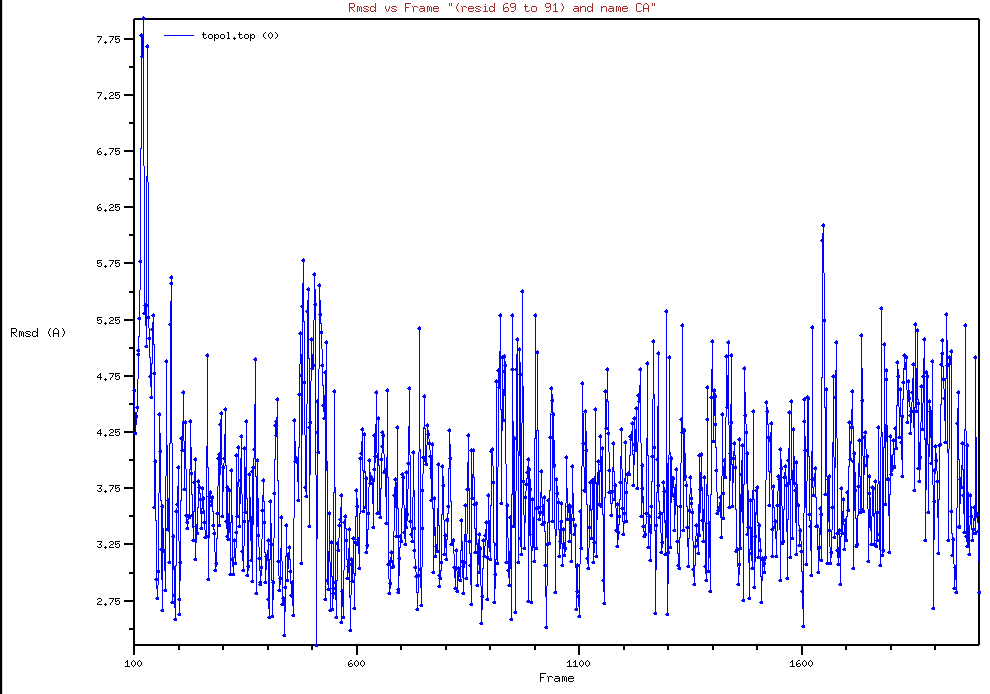
We can load these trajectory filed in any visualization tool to visualize the binding process step by step. Here we have added the lowest temperature trajectory trajectory.00.dcd (1000 frames due to size limit) as well as a screenshort showing rmsd of the peptide after aliging on the protein for the lowest temperature trajectory. Notice just slightly after 100 steps peptide finds the binding site with correct conformation and it stays there.
We can perform regular clustering on few low temperature replicas with cpptraj to find the most populated state which is our predicted native state. For this example have used hierarchical clustering with the script clustering.sh and the most population cluster and it’s comparision to the native structure is shown below:
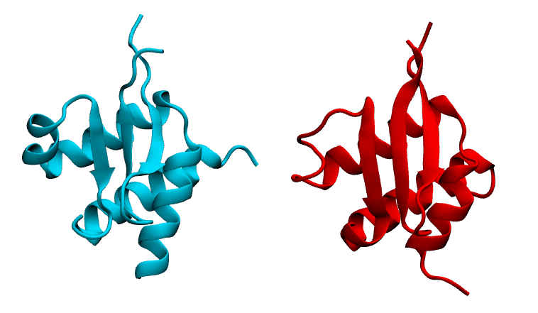
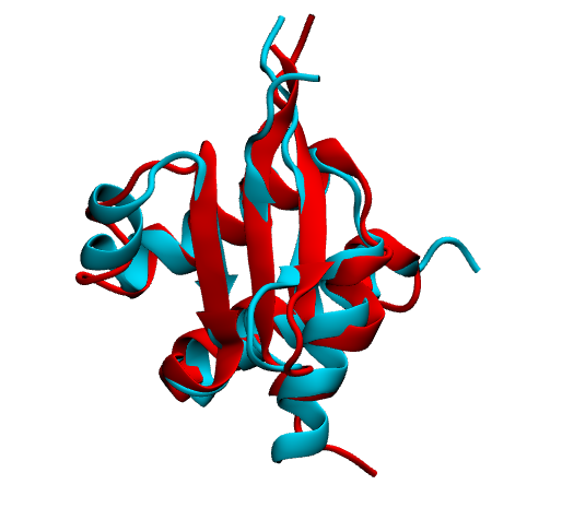
Here in the first image we are showing native in cyan and prediction (most populated cluster centroid) in red side by side. In the second image we are showing superimposition of them. Notice they prediction matches pretty well with native except the flexible loop region.
We can check if replica exchange is optimal in our simulation using the following commands:
analyze_remd visualize_trace
analyze_remd visualize_fup
Here are a couple of example of bad and good replica exchange:
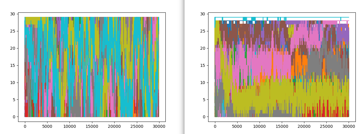
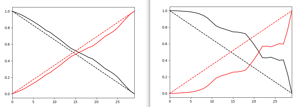
In both the example on the left, we have good exchange and on the right we have poor exchange. In the first image, different colors define different replicas. On the lest we see good mixing of them i.e. we have good exchnage among replicas and on the right mixing of colors is very poor suggesting a poor exchange.