Integrative modeling with cryo-EM data
In this tutorial, we describe how to set up simulation with cryo-EM data in MELD using adenylate kinase as an example.
Input preparation
To set up cryo-EM guided simulation in MELD, we first build the system given a PDB file.
Here we use the closed form of adenylate kinase (PDB: 1AKE) as the initial conformation.
For the target cryo-EM map, we use the generated density map from its open conformation (PDB: 4AKE).
We provide a gaussian kernel based density map builder pdb_map in process_density_map
process_density_map pdb_map -f ./4ake_t.pdb --map_save --sigma 2 -d .
where the sigma determines the simulated resolution of the map to be \(2*\sigma\). [1]
System setup
Now we can set up the simulation with the following:
N_REPLICAS = 8              #number of replicas
N_STEPS = 2000              #number of steps for each replica
BLOCK_SIZE = 20             #number of steps for saving trajectory

template = "./1ake_s.pdb"
p = meld.AmberSubSystemFromPdbFile(template)
build_options = meld.AmberOptions(
    forcefield="ff14sbside",
    implicit_solvent_model="gbNeck2",
    use_big_timestep=True,
    cutoff=1.8*u.nanometer
)
builder = meld.AmberSystemBuilder(build_options)
s = builder.build_system([p]).finalize()        #create system selected build options
s.temperature_scaler = meld.ConstantTemperatureScaler(300.0 * u.kelvin)     #set up temperature scaler
In this example, we use ff99SB force field with ff14sbside correction and gbNeck2 implicit solvent model. See Getting Started with MELD for more options.
Then we can add restraints based on density map to the system. Given a density map, a grid based potential can be defined as:
where \(\Phi(\mathbf{r})\) is the density value at position \(\mathbf{r}\), \(\Phi_{\mathrm{thr}}\) is the threshold for the density dataset to exclude solvent data with low density values. $zeta$ is a scale factor to control the strength of density map potential and also defines a flat potential for the solvent region. \(\Phi_{\max }=\max (\Phi(\mathbf{r}))\), which is designed to drive atoms into the high density region with low potential energy. The total energy \(\mathrm{t}\) of the system is given by \(U_\mathrm{t} = U_\mathrm{ff}+U_\mathrm{EM}+U_\mathrm{add}\), where \(U_\mathrm{EM} = \sum_{i} w_{i} V_{\mathrm{EM}}\left(\mathbf{r}_{i}\right)\) with \(w_{i}\) usually being the mass of atom \(i\) and \(U_\mathrm{add}\) can be additional restraints such as secondary structure restraints. For high resolution maps, we can smooth the generated grid potential by a Gaussian kernel to reduce the resolution of the map to alleviate the problem of atoms being trapped in a local minima of the rugged energy surface.
Following the replica exchange framework in MELD, we first create a blur_scaler
to blur the density map. Here we use a linear blur function to blur the map from 0 to 2 such that we will
use the original density map for the first replica and increasingly blur the map for the rest of replicas.
constant_blur is another option to define density map restraints with same blurring scale for all replicas.
The restraints can now be defined based on selected atoms in the system.
blur_scaler = s.restraints.create_scaler(
    "linear_blur", alpha_min=0, alpha_max=1,
    min_blur=0, max_blur=2, num_replicas=N_REPLICAS
)

for i in range(len(s.residue_numbers)):     #select non-hydrogen atoms in the system
    if "H" not in s.atom_names[i]:
        all_atoms.append(s.index.atom(resid=s.residue_numbers[i],atom_name=s.atom_names[i]))

density_map=s.density.add_density('./4ake_t_s2.mrc',blur_scaler,0,0.3)
r = s.restraints.create_restraint(
    "density",
    dist_scaler,
    LinearRamp(0,100,0,1),
    atom=all_atoms,
    density=density_map
)
map_restraints.append(r)
s.restraints.add_as_always_active_list(map_restraints)   #add restraints to the system
Next we can set up the parameters for replica exchange simulation.
# set run options with 100 steps for exchange and 100 steps for minimization
options = meld.RunOptions(
    timesteps = 100,
    minimize_steps = 100
)
# set up the data store
store = vault.DataStore(gen_state(s,0), N_REPLICAS, s.get_pdb_writer(), block_size=BLOCK_SIZE)
store.initialize(mode='w')
store.save_system(s)
store.save_run_options(options)

# create and store the remd_runner
l = ladder.NearestNeighborLadder(n_trials=100)
policy = adaptor.AdaptationPolicy(2.0, 50, 50)
a = adaptor.EqualAcceptanceAdaptor(n_replicas=N_REPLICAS, adaptation_policy=policy)

remd_runner = leader.LeaderReplicaExchangeRunner(N_REPLICAS, max_steps=N_STEPS, ladder=l, adaptor=a)
store.save_remd_runner(remd_runner)

# create and store the communicator
c = comm.MPICommunicator(s.n_atoms, N_REPLICAS)
store.save_communicator(c)

# create and save the initial states
states = [gen_state(s, i) for i in range(N_REPLICAS)]

store.save_states(states, 0)

# save data_store
store.save_data_store()
The complete script can be found here.
If the simulation is run on multiple GPUs, we can use mpirun -n 8 launch_remd --debug,
or we can use mpirun -n 1 launch_remd --debug to run the simulation on a single GPU.
Result analysis
After simulation is done, we can use extract_trajectory to extract frames
saved in Data/. The options can be seen from extract_trajectory --help
For example, we can extract frames from 1 to 200 of replica 0 in .dcd format.
extract_trajectory extract_traj_dcd --start 1 --end 200 --replica 0 trajectory.00.dcd
We can analyze the result based on the cross correlation between synthetic density maps of the simulation and target density map using
process_density_map pdb_map -f ./1ake_s.pdb -t trajectory.00.dcd -m ./4ake_c1.mrc --cc_save --cc -d .
From the correlation coefficient result, we can see that the initial conformation (blue) is progressively refined against the target map during the simulation. Representative conformation of high c.c. (yellow) is aligned against native structure (white).
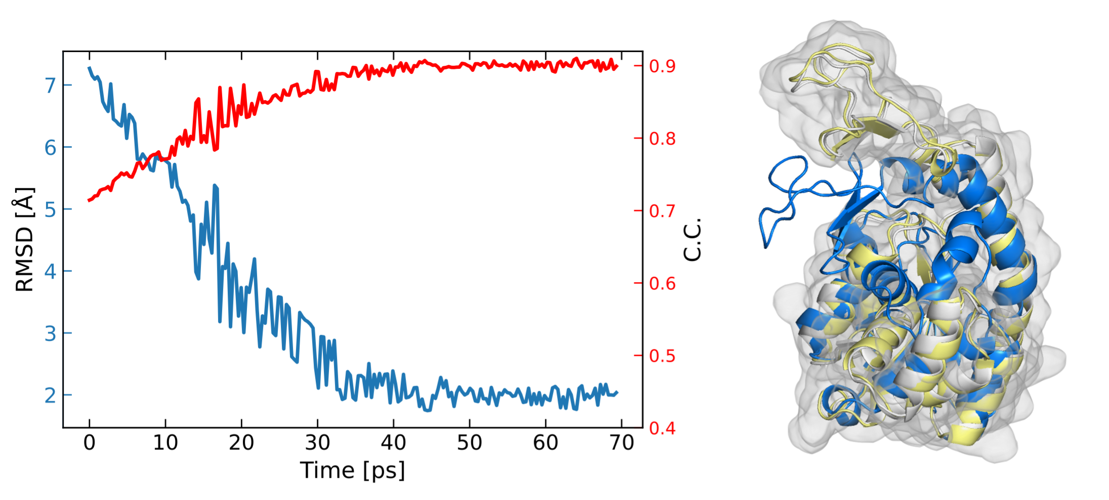
Correlation coefficient between synthetic density maps of simulation and target density map.